Basemap is a great library for mapping faster than other python options, but there are some usual things I couldn't find how to do. Clipping a raster using a shape is one of them. Here's how do I do it
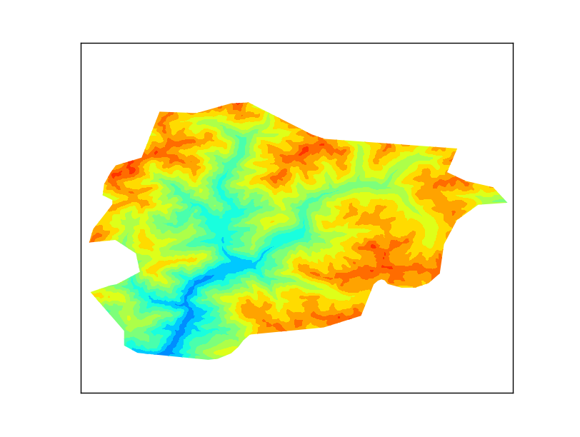 |
| The output |
As usual, all the code can be found at GitHub
Getting some data
The example plots some elevation data, taken from the SRTM. After looking for some options, the easiest to work with was this one: http://srtm.csi.cgiar.org/SELECTION/inputCoord.asp
The shapefile will be the border of Andorra, taken from Natural Earth
The result is a little poor because the resolution is low, but works well for the example.
The script
from mpl_toolkits.basemap import Basemap
from matplotlib.path import Path
from matplotlib.patches import PathPatch
import matplotlib.pyplot as plt
from osgeo import gdal
import numpy
import shapefile

fig = plt.figure()
ax = fig.add_subplot(111)

sf = shapefile.Reader("ne_10m_admin_0_countries")

for shape_rec in sf.shapeRecords():
    if shape_rec.record[3] == 'Andorra':
        vertices = []
        codes = []
        pts = shape_rec.shape.points
        prt = list(shape_rec.shape.parts) + [len(pts)]
        for i in range(len(prt) - 1):
            for j in range(prt[i], prt[i+1]):
                vertices.append((pts[j][0], pts[j][1]))
            codes += [Path.MOVETO]
            codes += [Path.LINETO] * (prt[i+1] - prt[i] -2)
            codes += [Path.CLOSEPOLY]
        clip = Path(vertices, codes)
        clip = PathPatch(clip, transform=ax.transData)


m = Basemap(llcrnrlon=1.4,
    llcrnrlat=42.4,
    urcrnrlon=1.77,
    urcrnrlat=42.7,
    resolution = None,
    projection = 'cyl')

ds = gdal.Open('srtm_37_04.tif')
data = ds.ReadAsArray()

gt = ds.GetGeoTransform()
x = numpy.linspace(gt[0], gt[0] + gt[1] * data.shape[1], data.shape[1])
y = numpy.linspace(gt[3], gt[3] + gt[5] * data.shape[0], data.shape[0])

xx, yy = numpy.meshgrid(x, y)

cs = m.contourf(xx,yy,data,range(0, 3600, 200))

for contour in cs.collections:
        contour.set_clip_path(clip)

plt.show()
- I used the pyshp library for reading the shapefile, since Fiona and GDAL don't work well together, and OGR was longer
- Lines 14 to 27 create the path. A Matplotlib path is made by two arrays. One with the points (called vertices in the script), and the other with the functions for every point (called codes)
- In our case, only straight lines have to be used, so there will be a MOVETO to indicate the beginning of the polygon, many LINETO to create the segments and one CLOSEPOLY for closing it
- Of course, only the polygon for Andorra has to be used. I get it from the shapefile attributes
- The prt array is for managing multipolygons, which is not the case, but the code will create correct clipping for multipolygons
- The path is created using the Path function, and then added to a PathPatch, to be able to use it as a closed polygon. Note the trasnform=ax.transData attribute. This assumes the polygon coordinates to be the ones used in the data (longitudes and latitudes in our case). More information here
- Next code lines draw the map as usual. I have used a latlon projection, so all the values for the raster and shapefile can be used directly. If the output raster was in an other projection, the shapefile coordinates should be appended to the path using the output projection (m(pts[j][0], pts[j][1]))
- The x and y coordinates are calculated from the GDAL geotransform, and then turned into a matrix using meshgrid
- The clipping itself is made in the lines 48 and 49. For each drawn element, the method set_clip_path is applied