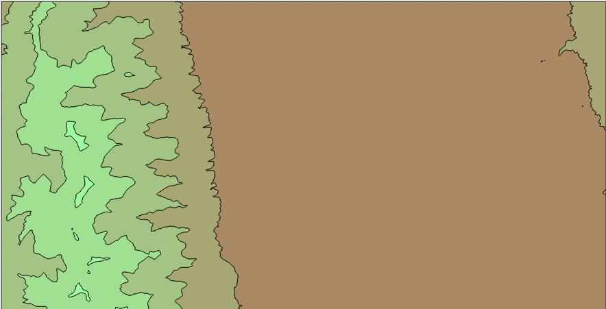
Unfortunately, there is no way to generate isobands, that is, filled contour lines that use polygons instead of polylines. Creating isobands allows the creation of nice contour maps easily, colouring the zones between two values:
Using contour lines, the result is this one:
Both visualizations are drawn directly from QGIS.
So I created two scripts to get the result. As usual, you can download them from
my GitHub account.
I created two scripts, since the one I like the most uses matplotlib, so sometimes it's not convenient to install. On the other hand, the other has less requirements (GDAL python), but the code is dirtier.
Both have the same usage, which is very similar to the
gdal_contour usage:
    Usage: isobands_matplotlib.py [-h] [-b band] [-off offset] [-i interval]
    [-nln layer_name] [-a attr_name] [-f formatname]
    src_file out_file
    Calculates the isobands from a raster into a vector file

    positional arguments:
      src_file         The raster source file
      out_file         The vectorial out file
    optional arguments:
      -h, --help       show this help message and exit
      -b band          The band in the source file to process (default 1)
      -off offset      The offset to start the isobands (default 0)
      -i interval      The interval (default 0)
      -nln layer_name  The out layer name (default bands)
      -a attr_name     The out layer attribute name (default h)
      -f formatname    The output file format name (default ESRI Shapefile)
Just choose the input and output files, the input file band to process (1 by default), and the interval, and you will get the vector file in the GIS format of your choice.
Now, the code of both script, step by step.
The script has a function called isobands, that actually generates the data, and a main part that reads the user input values:
if __name__ == "__main__":

    PARSER = ArgumentParser(
        description="Calculates the isobands from a raster into a vector file")
    PARSER.add_argument("src_file", help="The raster source file")
    PARSER.add_argument("out_file", help="The vectorial out file")
    PARSER.add_argument("-b",
        help="The band in the source file to process (default 1)",
        type=int, default = 1, metavar = 'band')
    PARSER.add_argument("-off",
        help="The offset to start the isobands (default 0)",
        type=float, default = 0.0, metavar = 'offset')
    PARSER.add_argument("-i",
        help="The interval  (default 0)",
        type=float, default = 0.0, metavar = 'interval')
    PARSER.add_argument("-nln",
        help="The out layer name  (default bands)",
        default = 'bands', metavar = 'layer_name')
    PARSER.add_argument("-a",
        help="The out layer attribute name  (default h)",
        default = 'h', metavar = 'attr_name')
    PARSER.add_argument("-f",
        help="The output file format name  (default ESRI Shapefile)",
        default = 'ESRI Shapefile', metavar = 'formatname')
    ARGS = PARSER.parse_args()

    isobands(ARGS.src_file, ARGS.b, ARGS.out_file, ARGS.f, ARGS.nln, ARGS.a,
        ARGS.off, ARGS.i)
I used the
argparse.ArgumentParser to read the script arguments, since is easy to use and it should come woth most of the updated python distributions (since python 2.7, I think).
This part of the code is quite easy to understand, it simply sets the arguments with their default value, sets if they are mandatory or not, etc.
The isobands function creates the vector file:
def isobands(in_file, band, out_file, out_format, layer_name, attr_name,
    offset, interval, min_level = None):
    '''
    The method that calculates the isobands
    '''
    ds_in = gdal.Open(in_file)
    band_in = ds_in.GetRasterBand(band)
    xsize_in = band_in.XSize
    ysize_in = band_in.YSize

    geotransform_in = ds_in.GetGeoTransform()

    srs = osr.SpatialReference()
    srs.ImportFromWkt( ds_in.GetProjectionRef() )

    #Creating the output vectorial file
    drv = ogr.GetDriverByName(out_format)

    if exists(out_file):
        remove(out_file)
    dst_ds = drv.CreateDataSource( out_file )

    dst_layer = dst_ds.CreateLayer(layer_name, geom_type = ogr.wkbPolygon,
        srs = srs)

    fdef = ogr.FieldDefn( attr_name, ogr.OFTReal )
    dst_layer.CreateField( fdef )


    x_pos = arange(geotransform_in[0],
        geotransform_in[0] + xsize_in*geotransform_in[1], geotransform_in[1])
    y_pos = arange(geotransform_in[3],
        geotransform_in[3] + ysize_in*geotransform_in[5], geotransform_in[5])
    x_grid, y_grid = meshgrid(x_pos, y_pos)

    raster_values = band_in.ReadAsArray(0, 0, xsize_in, ysize_in)

    stats = band_in.GetStatistics(True, True)
    if min_level == None:
        min_value = stats[0]
        min_level = offset + interval * floor((min_value - offset)/interval)

    max_value = stats[1]
    #Due to range issues, a level is added
    max_level = offset + interval * (1 + ceil((max_value - offset)/interval))

    levels = arange(min_level, max_level, interval)

    contours = plt.contourf(x_grid, y_grid, raster_values, levels)


    for level in range(len(contours.collections)):
        paths = contours.collections[level].get_paths()
        for path in paths:

            feat_out = ogr.Feature( dst_layer.GetLayerDefn())
            feat_out.SetField( attr_name, contours.levels[level] )
            pol = ogr.Geometry(ogr.wkbPolygon)


            ring = None

            for i in range(len(path.vertices)):
                point = path.vertices[i]
                if path.codes[i] == 1:
                    if ring != None:
                        pol.AddGeometry(ring)
                    ring = ogr.Geometry(ogr.wkbLinearRing)

                ring.AddPoint_2D(point[0], point[1])


            pol.AddGeometry(ring)

            feat_out.SetGeometry(pol)
            if dst_layer.CreateFeature(feat_out) != 0:
                print "Failed to create feature in shapefile.\n"
                exit( 1 )


            feat_out.Destroy()
- Lines 26 to 49 open the input file and create the output vector file.
- Lines 53 to 57 set two matrices, containing the coordinates for each pixel in the input file. To do it, two vectors are created first with the coordinates calculated from the input geotransform, and then the meshgrid is called to generate the 2d matrices, needed by matplotlib to make its calculations.
- Lines 59 to 70 read the input file data and calculates the levels inside it, from the interval and the offset. Since calculating isobands for levels not present in the file isn't efficient, the minimum and maximum values in the input file are calculated before the isobands.
- The line 72 is where the isobands are actually calculated using the contourf function.
- Lines 76 to 105 create the polygons at the output vector file.
- The generated contour has a property called collections, containing every isoband.
- Each element in the collections has the paths of the isolines.
- The property codes in the path indicates if a new ring has to be generated.
- The other lines are to generate an OGR feature
isobands_gdal.py
This script is quite dirtier, since I have used a trick to get the isobands from the ContourGenerate function.
Closing the contour lines, which is what has to be done to transform isolines to isobands, is not an easy task.
Looking at some D3js examples I got the idea from
Jason Davies conrec.js. I can't find the original example now, but basicaly, the idea is to add some pixels around the image with a value lower than the lowest value, so all the isolines will be closed. The solution gets closer, but some problems must be solved:
- Convert the isolines to polygons
- Clip the vectors to the original extent
- Substract the overlapping polygons, since when the lines are converted to polygons, all the area above the isoline value is contained in the polygon even though other lines with higher values are inside
 |
| When not clipped, the isolines will create strange effects at the borders |
The
main part code is exacly the same as in the other script, and the
isobands function is:
def isobands(in_file, band, out_file, out_format, layer_name, attr_name,
    offset, interval, min_level = None):
    '''
    The method that calculates the isobands
    '''
    #Loading the raster file
    ds_in = gdal.Open(in_file)
    band_in = ds_in.GetRasterBand(band)
    xsize_in = band_in.XSize
    ysize_in = band_in.YSize

    stats = band_in.GetStatistics(True, True)

    if min_level == None:
        min_value = stats[0]
        min_level = ( offset + interval *
            (floor((min_value - offset)/interval) - 1) )
    nodata_value = min_level - interval


    geotransform_in = ds_in.GetGeoTransform()

    srs = osr.SpatialReference()
    srs.ImportFromWkt( ds_in.GetProjectionRef() )

    data_in = band_in.ReadAsArray(0, 0, xsize_in, ysize_in)


    #The contour memory
    contour_ds = ogr.GetDriverByName('Memory').CreateDataSource('')
    contour_lyr = contour_ds.CreateLayer('contour',
        geom_type = ogr.wkbLineString25D, srs = srs )
    field_defn = ogr.FieldDefn('ID', ogr.OFTInteger)
    contour_lyr.CreateField(field_defn)
    field_defn = ogr.FieldDefn('elev', ogr.OFTReal)
    contour_lyr.CreateField(field_defn)

    #The in memory raster band, with new borders to close all the polygons
    driver = gdal.GetDriverByName( 'MEM' )
    xsize_out = xsize_in + 2
    ysize_out = ysize_in + 2

    column = numpy.ones((ysize_in, 1)) * nodata_value
    line = numpy.ones((1, xsize_out)) * nodata_value

    data_out = numpy.concatenate((column, data_in, column), axis=1)
    data_out = numpy.concatenate((line, data_out, line), axis=0)

    ds_mem = driver.Create( '', xsize_out, ysize_out, 1, band_in.DataType)
    ds_mem.GetRasterBand(1).WriteArray(data_out, 0, 0)
    ds_mem.SetProjection(ds_in.GetProjection())
    #We have added the buffer!
    ds_mem.SetGeoTransform((geotransform_in[0]-geotransform_in[1],
        geotransform_in[1], 0, geotransform_in[3]-geotransform_in[5],
        0, geotransform_in[5]))
    gdal.ContourGenerate(ds_mem.GetRasterBand(1), interval,
        offset, [], 0, 0, contour_lyr, 0, 1)

    #Creating the output vectorial file
    drv = ogr.GetDriverByName(out_format)
    if exists(out_file):
        remove(out_file)
    dst_ds = drv.CreateDataSource( out_file )


    dst_layer = dst_ds.CreateLayer(layer_name,
        geom_type = ogr.wkbPolygon, srs = srs)

    fdef = ogr.FieldDefn( attr_name, ogr.OFTReal )
    dst_layer.CreateField( fdef )


    contour_lyr.ResetReading()

    geometry_list = {}
    for feat_in in contour_lyr:
        value = feat_in.GetFieldAsDouble(1)

        geom_in = feat_in.GetGeometryRef()
        points = geom_in.GetPoints()

        if ( (value >= min_level and points[0][0] == points[-1][0]) and
            (points[0][1] == points[-1][1]) ):
            if (value in geometry_list) is False:
                geometry_list[value] = []

            pol = ogr.Geometry(ogr.wkbPolygon)
            ring = ogr.Geometry(ogr.wkbLinearRing)

            for point in points:

                p_y = point[1]
                p_x = point[0]

                if p_x < (geotransform_in[0] + 0.5*geotransform_in[1]):
                    p_x = geotransform_in[0] + 0.5*geotransform_in[1]
                elif p_x > ( (geotransform_in[0] +
                    (xsize_in - 0.5)*geotransform_in[1]) ):
                    p_x = ( geotransform_in[0] +
                        (xsize_in - 0.5)*geotransform_in[1] )
                if p_y > (geotransform_in[3] + 0.5*geotransform_in[5]):
                    p_y = geotransform_in[3] + 0.5*geotransform_in[5]
                elif p_y < ( (geotransform_in[3] +
                    (ysize_in - 0.5)*geotransform_in[5]) ):
                    p_y = ( geotransform_in[3] +
                        (ysize_in - 0.5)*geotransform_in[5] )

                ring.AddPoint_2D(p_x, p_y)


            pol.AddGeometry(ring)
            geometry_list[value].append(pol)


    values = sorted(geometry_list.keys())

    geometry_list2 = {}

    for i in range(len(values)):
        geometry_list2[values[i]] = []
        interior_rings = []
        for j in range(len(geometry_list[values[i]])):
            if (j in interior_rings) == False:
                geom = geometry_list[values[i]][j]

                for k in range(len(geometry_list[values[i]])):

                    if ((k in interior_rings) == False and
                        (j in interior_rings) == False):
                        geom2 = geometry_list[values[i]][k]

                        if j != k and geom2 != None and geom != None:
                            if geom2.Within(geom) == True:

                                geom3 = geom.Difference(geom2)
                                interior_rings.append(k)
                                geometry_list[values[i]][j] = geom3

                            elif geom.Within(geom2) == True:

                                geom3 = geom2.Difference(geom)
                                interior_rings.append(j)
                                geometry_list[values[i]][k] = geom3

        for j in range(len(geometry_list[values[i]])):
            if ( (j in interior_rings) == False and
                geometry_list[values[i]][j] != None ):
                geometry_list2[values[i]].append(geometry_list[values[i]][j])


    for i in range(len(values)):
        value = values[i]
        if value >= min_level:
            for geom in geometry_list2[values[i]]:

                if i < len(values)-1:

                    for geom2 in geometry_list2[values[i+1]]:
                        if geom.Intersects(geom2) is True:
                            geom = geom.Difference(geom2)

                feat_out = ogr.Feature( dst_layer.GetLayerDefn())
                feat_out.SetField( attr_name, value )
                feat_out.SetGeometry(geom)
                if dst_layer.CreateFeature(feat_out) != 0:
                    print "Failed to create feature in shapefile.\n"
                    exit( 1 )
                feat_out.Destroy()
- Lines 23 to 44 read the input file, including the data, geotransform, etc.
- Lines 47 to 54 create a vector file where the contour lines will be written. Since the data must be clipped later, the file is a temporary memory file.
- Lines 56 to 71 create a memory raster file with the input data, plus a buffer around it with a value lower than the lowest in the input data, so the contour lines will get closed.
- Line 74 calls the ContourGenerate function, that will add the contour lines to the vectorial memory file.
- Lines 77 to 91 create the actual output file
- Lines 93 to 130 create a collection of geometries with the polygons.
- The lines are transformed to polygons by creating a ring from the polyline and adding it to a polygon.
- Lines 113 to 123 clip the polygons to the original geotransform, by moving the coordinates of the points outside the geotransform to the border.
- Lines 138 to 167 stores the difference from the polygons that overlap, so the output polygons contain only the zones where the values are in the interval.
- Lines 170 to 187 write the final polygons to the output file, the same way than the other script.
Notes:
An other option would be, of course, creating the polygons myself. I tried to do it, but as you can see at the
marching squares wikipedia page, the algorithm is not easy when using polygons, and especially the matplotlib version of the scripts is quite clean.
The scripts have a problem when there is a nodata zone, since I haven't added the code to handle it.
Finally, as asked in the GDAL-dev mailing list, the best option would be modifying the ContourGenerate function to create isobands, but I think that is out of my scope.
The
discussion at the GDAL-dev mailing list where I posted the first version.
Some links I have used:
http://matplotlib.org/api/path_api.html
http://matplotlib.org/api/pyplot_api.html#matplotlib.pyplot.contourf
http://matplotlib.org/basemap/api/basemap_api.html#mpl_toolkits.basemap.Basemap.contourf
http://fossies.org/dox/matplotlib-1.2.0/classmatplotlib_1_1contour_1_1QuadContourSet.html


