D3 map Styling tutorial III: Drawing animated paths

The example La Belle France, or the original La Bella Italia by Gregor Aisch, have a nice ferry sailing along a path to connect the islands with the continent.
Drawing a path in a map, and animating some icon on it can be a nice tool to show information about routes, storm tracks, and other dynamic situations.

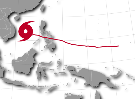
This example shows how to draw the Haiyan typhoon track on the map drawn in the last post.

The working examples are here:
Creating a geopath
Animating an object on the path

Getting the data

Both the base map data and the typhoon data are explained in the post  D3 map Styling tutorial I: Preparing the data

Creating a geopath

First, how to draw the path line on a map. The working example is here.

• The base map is drawn in the simplest way, as shown in this example, so the script stays clearer.
• The typhoon track is loaded from the json file generated in the first tutorial post (line 55)
• The path is created and inserted from lines 68 to 75:
• A d3.svg.line element is created. This will interpolate a line between the points. An other option is to draw segments from each point, so the line is not so smooth, but the actual points are more visible. 
• The interpolate method sets the interpolation type to be used.
• x and y methods, set the svg coordinates to be used. In our case, we will transform the geographical coordinates using the same projection function set for the map. The coordinates transformation is done twice, one for the x and another for the y. It would be nice to do it only once.
• The path is added to the map, using the created d3.svg.line, passing the track object as a parameter to be used by the line function. The class is set to path, so is set to a dashed red line (line 20)

Drawing the paths is quite easy, taking only two steps.

Animating an object on the path

 

The typhoon position for every day is shown on the path, with an icon. The icon size and color change with the typhoon class. The working example is here.

This second example is more complex than the first one:

• The base map has a shadow effect. See the second part of the tutorial for the source.
• The map is animated:
• Line 135 sets an interval, so the icon and line can change with the date.
• A variable i is set, so the array elements are used in every interval.
• When the dates have ended, the interval is removed, so everything stays quiet. Line 158.
• An icon moves along the path indicating the position of the typhoon
•  Line 128 created the icon. First, I created it using inkscape, and with the xml editor that comes with it, I copied the path definition. This method can get really complex with bigger shapes.
• Line 136 finds the position of the typhoon. The length of the track is found at line 122 with the getTotalLength() method.
• Line 137 moves the icon. A transition is set, so the movement is continuous even thought the points are separated. The duration is the same as the interval, so when the icon has arrived at the final point, a new transformation starts to the next one.
• Line 141 has the transform operation that sets the position (translate), the size (scale) and rotation (rotate). The factors multiplying the scale and rotation are those only to adjust the size and rotation speed. They are completely arbitrary.
• The path gets filled when the icon has passed. I made this example to learn how to do it. Everything happens at line 144. Basically, the trick is creating a dashed line, and playing with the stroke-dashoffset attribute to set where the path has to arrive.
• The color of the path and icon change with the typhoon class
• At line 54, a color scale is created using the method d3.scale.quantile. 
• The colors are chosen with colorbrewer, which is a set of color scales for mapping, and has a handy javascript library to set the color scales just by choosing their name. I learned how to use it with this example by Mike Bostock.
• The lines 156 and 142 change the track and icon colours.
• Finally, at line 154, the date is changed, with the same color as the typhoon and track.

Links

Simple path on a map - The first example
Haiyan typhoon track - The second example
D3 map Styling tutorial I: Preparing the data
D3 map Styling tutorial II: Giving style to the base map
Animated arabic kufic calligraphy with D3 - Animating paths using d3js
La Bella Italia - Kartograph example by Gregor Aisch
La Belle France - The same example as La Bella Italia, but using D3js
Every ColorBrewer Scale - An example to learn how to use ColorBrewer with D3js

Drawing wind barbs: GDAL python

Wind on a map is usually represented using wind barbs, a graphical way to show both speed and direction. The problem is that most GIS software is not prepared to draw them directly.
In this entry, I'll show how I use to generate PNG files from the meteorological model GFS, the same from the entry showing how to do some raster calculations.

As usual, the code is available at GitHub.

First the file that generates the png:

'''
Draws wind barbs on a png from a GRIB file using PIL
'''

import Image
import ImageDraw
from osgeo import gdal
from osgeo import osr
from osgeo.gdalconst import GA_ReadOnly
from math import floor
from math import ceil
from math import sqrt
from math import atan2
from math import degrees


def find_band_number(dataset, variable, level):
    '''
    Finds the band number inside the GRIB file, given the variable and the level names
    '''
    for i in range(1,dataset.RasterCount + 1):
        band = dataset.GetRasterBand(i)
        metadata = band.GetMetadata()
        band_level = metadata['GRIB_SHORT_NAME']
        band_variable = metadata['GRIB_ELEMENT']
        if (variable == band_variable) and (level == band_level):
            return i
    return None

def draw_barb(size, module, angle, color):
    extra_pixels = 10 #Avoid cutting the barb when rotating
    barb = Image.new('RGBA', (size + extra_pixels, size + extra_pixels))
    barb_draw = ImageDraw.Draw(barb)
    size = float(size) #Force it to float  
    separation = size/6
    module5 = int(round(module/5))

    x,v = divmod(module5,2)
    l,x = divmod(x,5)

    barb_draw.line([(extra_pixels,extra_pixels+size/2),(size+extra_pixels,extra_pixels+size/2)],color)
    pos = 0
    for nl in range(0,l,1): #50 kt triangles
        barb_draw.polygon([(extra_pixels+pos,extra_pixels+size/2),(extra_pixels+pos + extra_pixels+size/8,0),(extra_pixels+pos+size/4,extra_pixels+size/2),(extra_pixels+pos,extra_pixels+size/2)],color)

        pos = pos + size/4 + separation
    for nx in range(0,x,1):
        barb_draw.line([(extra_pixels+pos,extra_pixels+size/2),(extra_pixels+pos,extra_pixels+0)],color)

        pos = pos + separation
    if pos == 0: #advance a little for 5kt barbs
        pos = pos + separation
    if v == 1: # Only 0 or 1 are possible
        barb_draw.line([(extra_pixels+pos,extra_pixels+size/2),(extra_pixels+pos,extra_pixels+size/4)],color)

    barb = barb.rotate(angle, Image.BICUBIC)

    return barb

def draw_wind_barbs(xsize, ysize, out_file, data_file, epsg, geotransform, u_var, v_var, level, separation, barb_size, barb_color):
    out_img = Image.new('RGBA', (xsize, ysize) )

    dataset = gdal.Open(data_file, GA_ReadOnly )
    u_band_id = find_band_number(dataset, u_var, level)
    v_band_id = find_band_number(dataset, v_var, level)

    band_u = dataset.GetRasterBand(u_band_id)
    band_v = dataset.GetRasterBand(v_band_id)

    geotransform_in = dataset.GetGeoTransform()   

    xsize_in = band_u.XSize
    ysize_in = band_u.YSize

    values_u = band_u.ReadAsArray(0, 0, xsize_in, ysize_in)
    values_v = band_v.ReadAsArray(0, 0, xsize_in, ysize_in)
    

    proj_in = osr.SpatialReference()
    proj_in.SetFromUserInput(dataset.GetProjection())
    proj_out = osr.SpatialReference()
    proj_out.ImportFromEPSG(epsg)

    transf = osr.CoordinateTransformation(proj_out,proj_in)

    for px in range(0,xsize + separation,separation):
        x_out = geotransform[0] + px * geotransform[1]
        for py in range(0,ysize + separation,separation):
            y_out = geotransform[3] + py * geotransform[5]
            point = transf.TransformPoint(x_out, y_out,0)
            px_in = (float(point[0]) - geotransform_in[0]) / geotransform_in[1]
            py_in = (float(point[1]) - geotransform_in[3]) / geotransform_in[5]
           
            d1 = 1/sqrt( pow((px_in - floor(px_in)), 2) + pow((py_in - floor(py_in)), 2) )
            d2 = 1/sqrt( pow((ceil(px_in) - px_in), 2) + pow((py_in - floor(py_in)), 2) )
            d3 = 1/sqrt( pow((ceil(px_in) - px_in), 2) + pow((ceil(py_in) - py_in), 2) )
            d4 = 1/sqrt( pow((px_in - floor(px_in)), 2) + pow((ceil(py_in) - py_in), 2) ) 
            d_sum = d1 + d2 + d3 + d4   

            u = (d1*values_u[floor(py_in)][floor(px_in)] + d2*values_u[floor(py_in)][ceil(px_in)] + d3*values_u[ceil(py_in)][ceil(px_in)] + d4*values_u[ceil(py_in)][floor(px_in)]) / d_sum
            v = (d1*values_v[floor(py_in)][floor(px_in)] + d2*values_v[floor(py_in)][ceil(px_in)] + d3*values_v[ceil(py_in)][ceil(px_in)] + d4*values_v[ceil(py_in)][floor(px_in)]) / d_sum

            module = 1.943844494 * sqrt((u*u)+(v*v)) #in knots
           
            angle = degrees(atan2(v,u)) #Angle like in trigonometry, not wind direction where 0 is northern wind
            try:
                barb = draw_barb(barb_size, module, angle, barb_color)
                out_img.paste(barb, (px-(barb_size/2),py-(barb_size/2)), barb)
            except Exception, ex:
                raise Exception("No es pot dibuixar la barba: " + str(ex))
   
    out_img.save( out_file )

    #Creating the pngw worldfile
    fp = open(out_file.replace("png","pngw"),"w")
    print str(geotransform[1])+"\n0\n0\n"+str(geotransform[5])+"\n"+str(geotransform[0])+"\n"+str(geotransform[3])
    fp.write(str(geotransform[1])+"\n0\n0\n"+str(geotransform[5])+"\n"+str(geotransform[0])+"\n"+str(geotransform[3]))
    fp.close()

if __name__ == '__main__':
   
    draw_wind_barbs(600, 400, 'wind.png', 'gfs_3_20130524_0000_000.grb', 4326, [0, 0.1, 0, 70, 0, -0.1], 'UGRD', 'VGRD', '850-ISBL', 20, 20, '#000000')

• The last part of the file (line 122) shows how to call tha main function draw_wind_barbs
• draw_wind_barbs takes the following arguments:
• xsize, ysize: The output image size
• out_file: the output png file. An other file will be created with the extension pngw, as the worldfile.
• data_file: The input file from the model (actually, any GRIB file with the wind in U and V components)
• epsg, geotransform: The output projection parameters.
• u_var, v_var, level: The wind component variable names (south-north is v, east-west is u) as they appear in the GRIB_ELEMENT metadata in the GRIB file. Level as it appears in the GRIB_SHORT_NAME metadata.
• separation, barb_size, color: The separation and size in pixels at the output file (it's possible change the barb density)
• From line 61 to 84, the function creates the output image according to the input file features and the output file as asked in the parameters
• The number of the band corresponding to the u and v components is calculated with the function find_band_number, that looks into the file metadata to match the asked values with some of the existing bands. Lines 17-28
• From 86 to 110, the barbs are drawn. For every n pixels as asked in the separation parameter, a barb is calculated. To do it, is necessary to know the position in the input file (lines 91 to 98), with the projection transformation,
• Then the wind value is calculated from the closest four pixels in the original file, using the inverse of the distance method . lines 94-102
• After the u and v components are known, the module and angle are calculated. Note that the original speeds are in m/s, but the barbs use knots, so the transformation is done here.The angle is not S-N, but W-E, which is fine for drawing, but a bit confusing. The coordinates origins are S and W.
• With the angle and module, the barb can be drawn, using the function draw_barb, and the result pasted into the output file.
• The draw_barb function divides the module by 5, 10 and 50 to know how many ticks the barb has to have, and draws the barb with the PIL polygon and line methods.
• The file is written and the worldfile is created at lines 114-118

To download the data files and draw directly the png, I wrote the following script:

from urllib2 import urlopen
from urllib2 import HTTPError
from sys import exit
from datetime import datetime
from barbs import draw_wind_barbs

def download_file(year,month,day,hour,valid_time):
    filename = "gfs_3_%d%02d%02d_%02d00_%03d.grb"%(year, month, day, hour, valid_time)
    url = "http://nomads.ncdc.noaa.gov/data/gfs-avn-hi/%d%02d/%d%02d%02d/gfs_3_%d%02d%02d_%02d00_%03d.grb"%(year, month, year, month, day, year, month, day, hour, valid_time)
    try: 
        req = urlopen(url)
    except HTTPError:
        print "File not found: May be the date is incorrect?"
        exit()

    f = open(filename, 'w')
    f.write(req.read())
    f.close()
    return filename

if __name__ == "__main__":
    now = datetime.now()
    print now.year
    year = raw_input('Type year ('+str(now.year)+'): ')
    month = raw_input('Type month ('+str(now.month)+'): ')
    day = raw_input('Type day ('+str(now.day)+'): ')
    hour = raw_input('Type hour (0): ')
    valid_time = raw_input('Type valid time (0): ')
    if (year == ''):
        year = now.year
    if (month == ''):
        month = now.month
    if (day == ''):
        day = now.day  
    if (hour == ''):
        hour = 0
    if (valid_time == ''):
        valid_time = 0     
    filename = download_file(int(year),int(month),int(day),int(hour),int(valid_time))
    out_filename = filename.replace("grb","png")

    draw_wind_barbs(600, 400, out_filename, filename, 4326, [0, 0.1, 0, 70, 0, -0.1], 'UGRD', 'VGRD', '850-ISBL', 20, 20, '#000000')

• The main part takes the date wanted by the user and sets it at the current day at 00h as default. 
• After that, calls the download_file function to download the GRIB file from the server.
• Then call the draw_wind_barbs function to draw the map. Try changing the geotransform and image size to see how the output changes.

Finally, to draw the file with the map at the background, I have  opened the png with QGIS (since it has the worldfile, is possible to do it), and added the background from naturalearth before exporting the image as a png.

Raster calculations with GDAL and numpy: calculating GFS wid speed

Performing raster calculations is a frequent need. GDAL python bindings come with a utility program,  gdal_calc.py, that does that, but many times is useful to code them.

In this example, we will be able to calculate the wind speed field from the GFS model, from the given u and v speed.

 The calculated wind field. America is easily seen at the right side of the image

The data

In this example, we will use the GFS global model data, which is available at their web site. Just navigate to a date that pleases you and download a .grb file.

Files are in grib format, with a little problem when trying to view them in QGis: Coordinates are from 0 to 360º in longitude, while the usual thing is to put them from -180º to 180º. Everything will work without changing this, but you can do it after taking a look to this post.

Inside the grib file, there are many bands (hundreds). You can see their definition using the gdal command gdalifo, or the file with the extension *inv at the same place you downloaded the grib file. There are many wind fields, that correspond to different altitudes, all them indicated as u (east) and v components (north). Just take note of the band number of both at the desired level.

NumPy

The best of using the python gdal bindings, compared from those of the other programs, is that converting a raster file to a NumPy matrix is now very easy. 

NumPy is a python extension that allows to perform matrix calculations in a really easy and efficient way. It should be installed in your computer if GDAL python is installed.

Once you have two matrices A and B in NumPy, adding element by element to a C matrix would be as easy as:

C = A + B

and multiplying:

C = A * B

Note that is not a matrix multiplication (more info here), but this is what we usually need when working with raster images.

The code

The wind speed is the modulus of the two components, so 

spd = sqrt(u^2+v^2)

The "traditional way" to calculate it would be opening two bands and loop all the elements to create the new band. Instead, this can be done:

from osgeo import gdal
from osgeo.gdalnumeric import *
from osgeo.gdalconst import *

fileName = "gfs.tiff"
bandNum1 = 199
bandNum2 = 200

outFile = "out.tiff"

#Open the dataset
ds1 = gdal.Open(fileName, GA_ReadOnly )
band1 = ds1.GetRasterBand(bandNum1)
band2 = ds1.GetRasterBand(bandNum2)

#Read the data into numpy arrays
data1 = BandReadAsArray(band1)
data2 = BandReadAsArray(band2)

#The actual calculation
dataOut = numpy.sqrt(data1*data1+data2*data2)

#Write the out file
driver = gdal.GetDriverByName("GTiff")
dsOut = driver.Create("out.tiff", ds1.RasterXSize, ds1.RasterYSize, 1, band1.DataType)
CopyDatasetInfo(ds1,dsOut)
bandOut=dsOut.GetRasterBand(1)
BandWriteArray(bandOut, dataOut)

#Close the datasets
band1 = None
band2 = None
ds1 = None
bandOut = None
dsOut = None

Note that:

1. gdalnumeric is used, because it's the easiest way to dump a raster into a NumPy matrix using BandReadAsArray and the inverse function with BandWriteArray.
2. In this case, we are reading the bands 199 and 200, but you should check which bands are the ones to read in the file you download.
3. CopyDatasetInfo will copy all the input file metadata into the output file. This includes the geotransform, the projection, the GCPs (there aren't in this case) and the other metadata.
4. Don't forget to set the bands and datasets to None at the end to free them. In longer scripts this may be critical.

gdal_calc.py

If you want to use the command line function to do the same, you can try with:

gdal_calc.py -A gfs.tiff --A_band 199 -B gfs.tiff --B_band 200 --outfile out.tiff --calc="sqrt(A*A+B*B)"

It gives the same result.